Ultrasound imaging is widely used in hospitals to produce pictures of inside a patient’s body. It is commonly used to examine unborn babies in pregnant women and to diagnose certain conditions. An ultrasound transducer is used to generate high-frequency pulses of sound which reflect off the different tissue layers present in a body. The reflected sound waves are received by the same transducer and post-processed to create an image in real-time. It is important to understand each element of the physics being modelled to determine how much complexity is required for a useful result. In this post, we explore some of the considerations routinely encountered by our engineers.
Why is modelling an ultrasound transducer challenging?
Ultrasound transducers are typically constructed from an array of piezoelectric crystals (red) mounted on a backing material (yellow) with an acoustic matching layer (green) and lense (blue).
Transducer construction and mesh strategy
A model needs to simulate electrical excitation of the crystal, propagation of the resulting waves and their transduction back into an electrical signal. A multiphysics problem. These components are built on the scale of an acoustic wavelength, with even smaller discrete mesh elements needed to resolve the waves. A transient simulation on this mesh requires small time steps to solve, a constraint known as the CFL condition. If the waves generated travel beyond a mesh element following a single time step their true behaviour will not be captured. The physical degrees of freedom, geometric details and time steps required to produce a serious computational challenge.
How can we simplify the problem?
In many cases, it is useful to consider the same approaches to simplification. Can a degree of symmetry be exploited? Can a simpler mathematical formulation be used? Can we truncate the domain being simulated? The answer to these questions is often application-specific and depends on the experience of an engineer. Let’s consider a beam steered transducer model where symmetry is not a possibility. A simple pressure acoustic formulation could be attempted, but the contribution of shear waves may not be understood. Truncating the backing material – which makes up most of the model – is an option that can greatly reduce the model complexity.

By using a low reflecting boundary where we perform our “cut” we can absorb both pressure and shear waves, giving us the response of a much thicker layer without the overhead.
Results
The figures below display pressure and shear waves, simulated for both the full and truncated models. Waves are displayed travelling from the crystal in both the left and right directions, the former being absorbed by the backing.


We observe damping of both pressure and shear waves in the backing with a full model, as designed. This behaviour is replicated for both waves with the truncated model, with minimal reflection observed from the low reflecting boundary. The solving time on a 16-core AMD Threadripper 1950X is halved, from 10 minutes to less than 5 minutes. This improvement becomes substantial when we consider the exploration of realistic transducer arrays with over 128 elements. The addition of an acoustic target volume results in a modest solve time increase to 7.5 minutes (constant with respect to array size), producing the following figure where time delays have been introduced to steer the beam.

Other techniques to consider
Very large models which extend into 3D can render unviable the solid mechanics approach presented here. In such cases, an acoustic approximation or an elastic wave formulation could provide the required detail.
What we used to make these models
The models presented here used COMSOL Multiphysics with the following interfaces:
Electrostatics
Solid Mechanics
Acoustics
Why choose Xi for your next project
We are a team of engineers with broad industrial experience – from the acoustics of electrostatic headphones to seismic vibrations from wind turbines. The simulation approach discussed above is applicable to situations where the physical size of objects is comparable to the wavelength under consideration. Examples include the analysis of beam steered acoustic speakers/microphones and ground-borne vibrations.