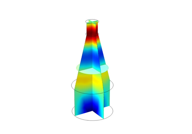
Transducer design optimisation
Xi Engineering Consultants modelled and optimised a piezoelectric transducer for structure borne data transmission, delivering a robust, low risk design that works where electromagnetic communication fails.

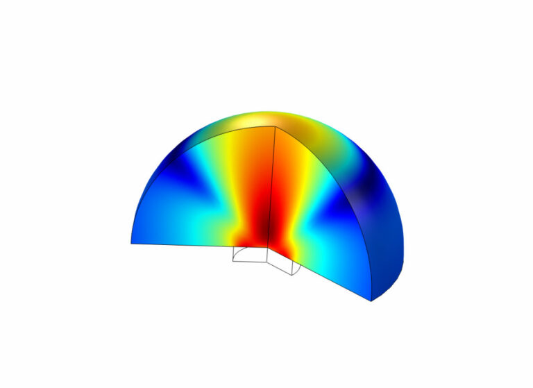
Xi Engineering Consultants modelled and optimised a piezoelectric transducer for structure borne data transmission, delivering a robust, low risk design that works where electromagnetic communication fails.
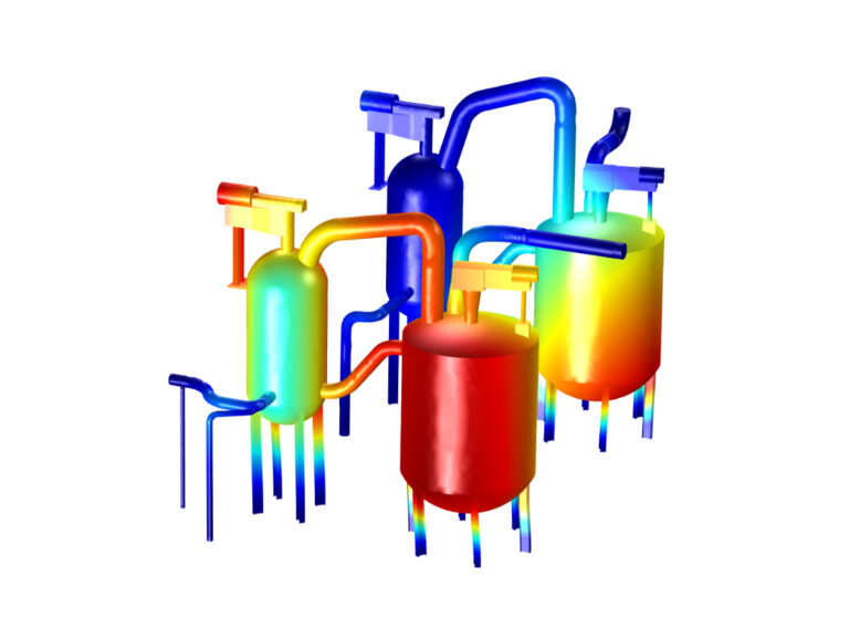
Xi Engineering Consultants measured and modelled vibration in a refinery agitator building, pinpointed fatigue hot spots and recommended targeted structural upgrades to protect pipework and steelwork from vibration induced failure.
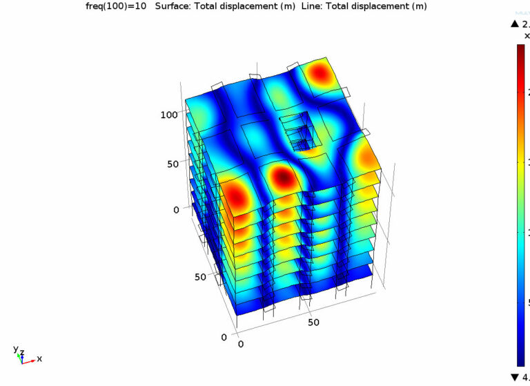
Xi Engineering Consultants uses targeted measurement and simulation to diagnose structural vibration problems and design practical mitigation, protecting comfort and sensitive equipment in demanding buildings.
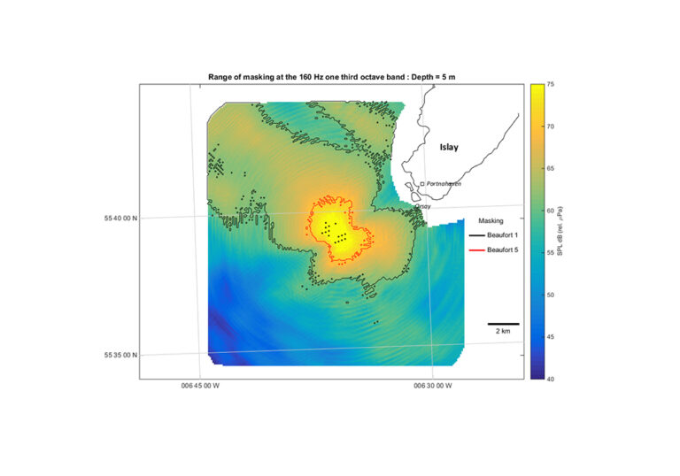
Xi Engineering Consultants modelled underwater noise from a 30 MW tidal array off Islay and assessed species specific impacts, helping DP Energy secure Marine Scotland consent.
Xi Engineering Consultants simulated the smart home device’s microphone chamber, checking resonances and thermoviscous losses so the client could commit to tooling with confidence in voice activation performance.
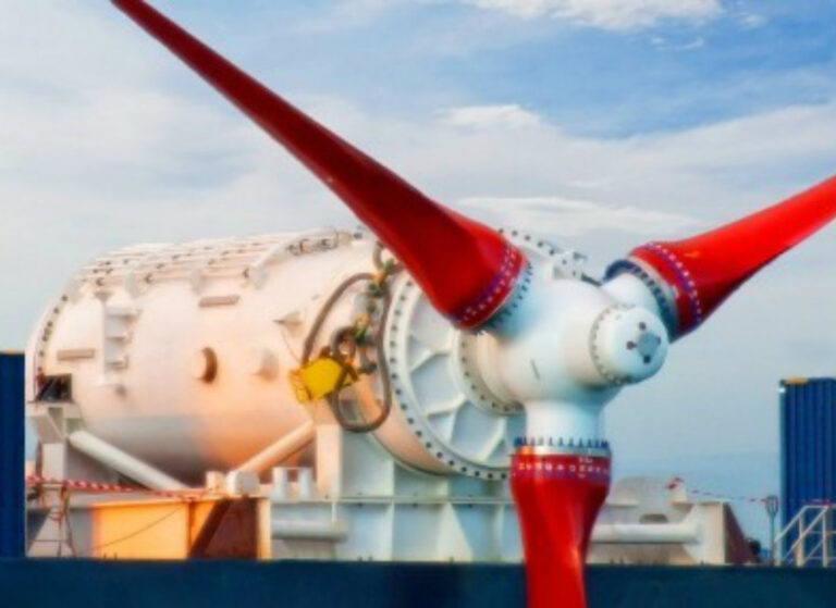
Xi Engineering Consultants built holistic dynamic models for Andritz Hydro Hammerfest’s tidal turbines, optimising designs for fatigue and resonance and reducing the need for costly offshore prototypes.

Xi Engineering Consultants created calibrated Multiphysics models of Warwick Acoustics’ electrostatic headphone transducers, cutting prototype builds, optimising performance and enabling rapid customisation for end clients.

Xi Engineering Consultants built a MATLAB based tool for Edge Mobility that turns custom motorcycle drive cycles into power and torque profiles, helping engineers size electric motors accurately and quickly.
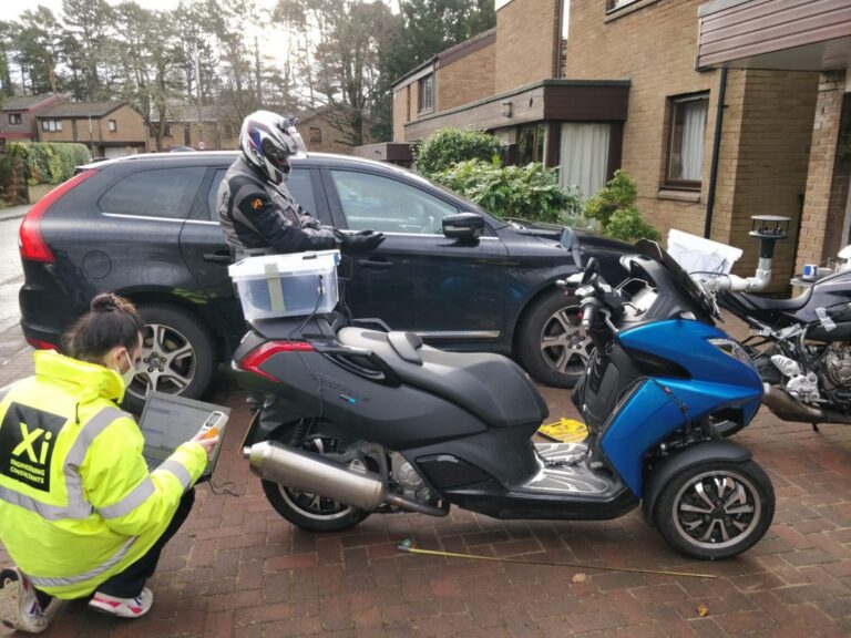
Xi Engineering Consultants instrumented a motorcycle with GPS, motion and wind sensors to measure real drive cycles, using the data to validate and refine a power and torque model for electric bike design.
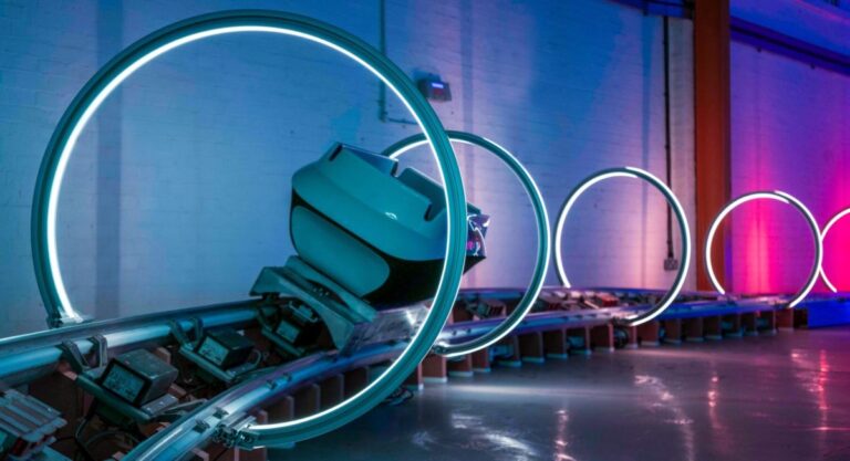
Xi Engineering Consultants supports Magway’s all electric goods delivery system with Multiphysics simulation and digital twin development, validating designs, reducing risk and speeding up commercial deployment.