Where is ultrasonic non-destructive testing used?
From offshore wind turbines, desalination plants, bridges and rail lines, to boats, aircraft motors, pipelines and our own bodies, maintenance is a (hopefully) boring but essential topic. Structures are subjected to a huge range of environmental influences that may cause damage or improper functioning. Continuous steady winds, as well as the occasional strong gusts, can strain drive shafts and wear down teeth in wind turbine gearboxes. Extreme temperatures and combustion processes may directly damage surfaces within an aircraft engine over time and thermal expansion will contribute to material fatigue. Fouling of filtration membranes in reverse osmosis (RO) desalination plants clog up the system and make it unable to continue processing seawater. And all manner of maladies such as cancerous tumours, hernias, internal lesions, or joint damage can afflict us personally. All of these “stressors” and “defects” are things that indicate a problem with the system and the need to undertake active remedial measures, whether that be cleaning, re-machining, part replacement, or even surgery.

Figure 1: All kinds of systems and their constituent parts undergo wear and tear, and they periodically need maintenance or replacing.
One thing all of these examples have in common is that the defects are often invisible to the naked eye, especially when they are first developing. In cases of structural fatigue, failure often starts with the formation and growth of cracks. Cracks may form on the surface or deep within a structure; weld joints, for example, are particularly prone to crack formation. Crack growth often starts slowly but may unpredictably and suddenly lead to catastrophic failure.
So how are we to identify these problems before they become problems? You can’t simply drive heavier and heavier trucks over a small bridge until it falls down, and then declare the structural issue solved. This is where non-destructive testing and monitoring comes in and using ultrasound is one of the most straightforward and common ways to do this.
How does ultrasonic non-destructive testing work?
Fundamentally, the concept behind ultrasonic non-destructive testing (NDT) is quite simple. We generate a sound, send it out, and listen for the echo. By listening to the echo, we can learn about the objects the sound bounced off of. Sonar, as used by bats or vessels at sea, is one form of this. Ultrasonic NDT for structural analysis or medical imaging follows a similar concept, but usually at much higher frequencies – typically in the MHz range. Such high frequencies produce acoustic waves with very small wavelengths, which allows you to resolve very small structures or defects; these can be cracks, fouling layers on a filtration membrane, damage to the meniscus in your knee, or corrosion in a pipe.
The sound waves are generated by an ultrasonic transducer, the core of which is a piezoelectric element. Piezoelectric elements are interesting materials because when you apply a voltage to them, they physically expand and contract. So, if you put a voltage pulse across the piezoelectric element, it will expand and contract, displacing the material next to it and sending out a wave.
Conversely, when an external wave impacts the piezoelectric element, a voltage is generated and can be measured. This allows the element to function both as a generator and as a detector of sound.
If the piezoelectric element is used to send out a pulse, the pulse will reflect off of interfaces with other materials, and the echo may return to the transducer. Upon returning, the echo itself (a pressure wave) imposes a mechanical stress on the element, generating a terminal voltage. This simple configuration is called an A-Scan. A COMSOL simulation is shown in Figure 3, where a pressure pulse is generated by a transducer; it travels through a plastic block (called a delay line), through an aluminium wall and into water. This might represent, for example, a reactor system for an industrial chemical process.
Recording returning echoes is a technique that is often used for calculating the distance of objects below the surface, such as for measuring the wall thickness here. If you know the speed of sound in the material and the return time of the echo, it’s easy to calculate the distance.
The reason such echoes occur is because of differences in a material property called the acoustic impedance. In an isotropic material, this material property is simply equal to the product of the density and the speed of sound. At locations where there is an interface and a difference in the acoustic impedance, some portion of the wave will be transmitted, and some will be reflected. The part that is reflected hits the ultrasonic transducer and is recorded as a voltage pulse.
When an acoustic wave is incident on a surface at an angle, things can get a bit complicated, with reflections, transmissions, and the transformation of waves from longitudinal waves to shear waves. That’s a topic for another day.
The voltage vs. time shown in Figure 3 is a representation of Ultrasonic Time-Domain Reflectometry at a single point (A-scan). Expanding upon this concept, you can characterize wall thickness (or any other buried features) along a path, by simply moving the transducer left/right (B-scan), or over a surface by moving the transducer left/right and up/down (C-scan). The surfaces, of course, don’t have to be flat; many transducers can be outfitted with delay lines that have a curved surface, allowing fitting to pipes of different diameters, for example. The refraction due to the curved surface is then accounted for in signal processing.
Scans can be carried out by physically moving a single-element transducer, or alternatively, with a single sensor head containing an array of transducers mounted at a fixed location. By correctly timing when each element in the array triggers a pulse, the series of waves emitted will constructively and destructively interfere, forming a beam in a specified direction. This is called beam steering and is performed by phased-array transducers; it is powerful technique and allows the user a large degree of flexibility in performing maintenance surveys. Indeed, most medical imaging systems are built on a form of this.


Figure 2: A COMSOL simulation of a simple piezoelectric element, with a voltage pulse applied at the terminal. The piezoelectric material deforms (exaggerated here for visualization) and emits pressure waves into the surrounding material.


Figure 3: Top: ultrasonic pulse reflecting off of interfaces between different materials: plastic/aluminium and aluminium/water. Note that there are multiple secondary internal reflections. The echoes can be seen in the terminal voltage plot, occurring at different return times, according to the distance and speed of sound in the materials.

Figure 4: The concept of phased-array transducers for ultrasonic NDT (from https://en.wikipedia.org/wiki/Phased_array_ultrasonics).
Modelling of ultrasonic non-destructive testing using COMSOL Multiphysics
A good basic application example involves using ultrasonic non-destructive testing for monitoring fouling or corrosion in pipes or flow-channels in fluid processing equipment. This can be found, for example in oil refinement, agriculture, municipal water delivery, chemical processing, or desalination.
Sediments in the fluid or organic matter may deposit on the wall over time. Organic matter in particular may grow, forming a thick slime known as biofouling. Arteries are also another common flow system that may clogged up, for example, and can be monitored with medical ultrasound. Ultrasonic NDT can help monitor all of these cases in a cost-effective way. In the end, layers of material with differing acoustic properties are present, and reflected echoes are recorded and analysed.


Figure 5: An ultrasonic transducer mounted to the wall of a manifold used in a fluid processing application. Top: A flat fouling layer has formed between the wall and the water. Bottom: the inner wall is corroded. Note how the type and shape of the interface affects the shape of the of the reflected and transmitted waves.
We can look at the transducer voltage to see if we can make out the differences between the signals reflected from a clean wall, a wall with fouling layers of different thickness, or a corroded wall.

Figure 6: Plot of different recorded echoes, zoomed in around the time when echoes return to the transducer.
That looks like a mess! But there are a few things we can immediately say about these signals. First, there clearly are differences between the waveforms recorded for each wall condition. Second, all of the signals overlap up until about 13 µs. So, the first echo, off of the delay-line/wall interface, is the same for all cases but there’s something different about the echoes that follow.
There are many possible ways to further investigate the differences in these signals. In particular, we’re interested to see if there’s something clearly different between a fouled wall and a corroded wall, or between walls with different fouling thickness. One basic way to start is by looking at the difference between each of these signals and a reference signal. A natural reference signal is the one from the case where the wall is known to be clean. Below we show plots of a normalized root mean square (RMS) difference between each signal and the “clean” signal (at all points), and then we look at the cumulative difference over the full echo recorded time span.

Figure 7: Top: A plot of the pointwise normalized root mean square (RMS) difference between each signal and the reference signal (clean wall). Bottom: Cumulative difference over the echo return timespan.
Here, clearer patterns emerge. Again, there are no differences between the signals up to about 13 µs, but after that, the corroded wall shows a bigger change than the fouled walls. This is pretty clear in both the difference-factor and cumulative-difference-factor plots. The cumulative-difference-factor plot, however, does help us see that the thin fouling layer (1 mm) can be clearly distinguished from the two thicker layers (2 mm, 4mm). The two thicker layers are more difficult to distinguish from each other, but produce a bigger “difference”, with respect to the “clean” signal.
Xi Engineering’s expertise and capabilities
Xi Engineering has extensive experience in the analysis of acoustics in a wide range of applications, including ultrasonic non-destructive testing (NDT), high-end headphone design, sound damping in the built environment, vibrations affecting sensitive scientific equipment, and wind farm planning/consent, to list a few.
If you have a project where the propagation of sound waves is a key concern, we can help in developing mathematical models using numerical software packages such as COMSOL Multiphysics to accelerate your innovation.